Alpha diversity

Part 1: Alpha diversity main measures.

dataset: phyloseq

The diet swap data set represents a study with African and African American groups undergoing a two-week diet swap. For details, see https://www.nature.com/articles/ncomms7342.

phyloseq-class experiment-level object
otu_table()   OTU Table:         [ 130 taxa and 222 samples ]
sample_data() Sample Data:       [ 222 samples by 8 sample variables ]
tax_table()   Taxonomy Table:    [ 130 taxa by 3 taxonomic ranks ]

Boxplots

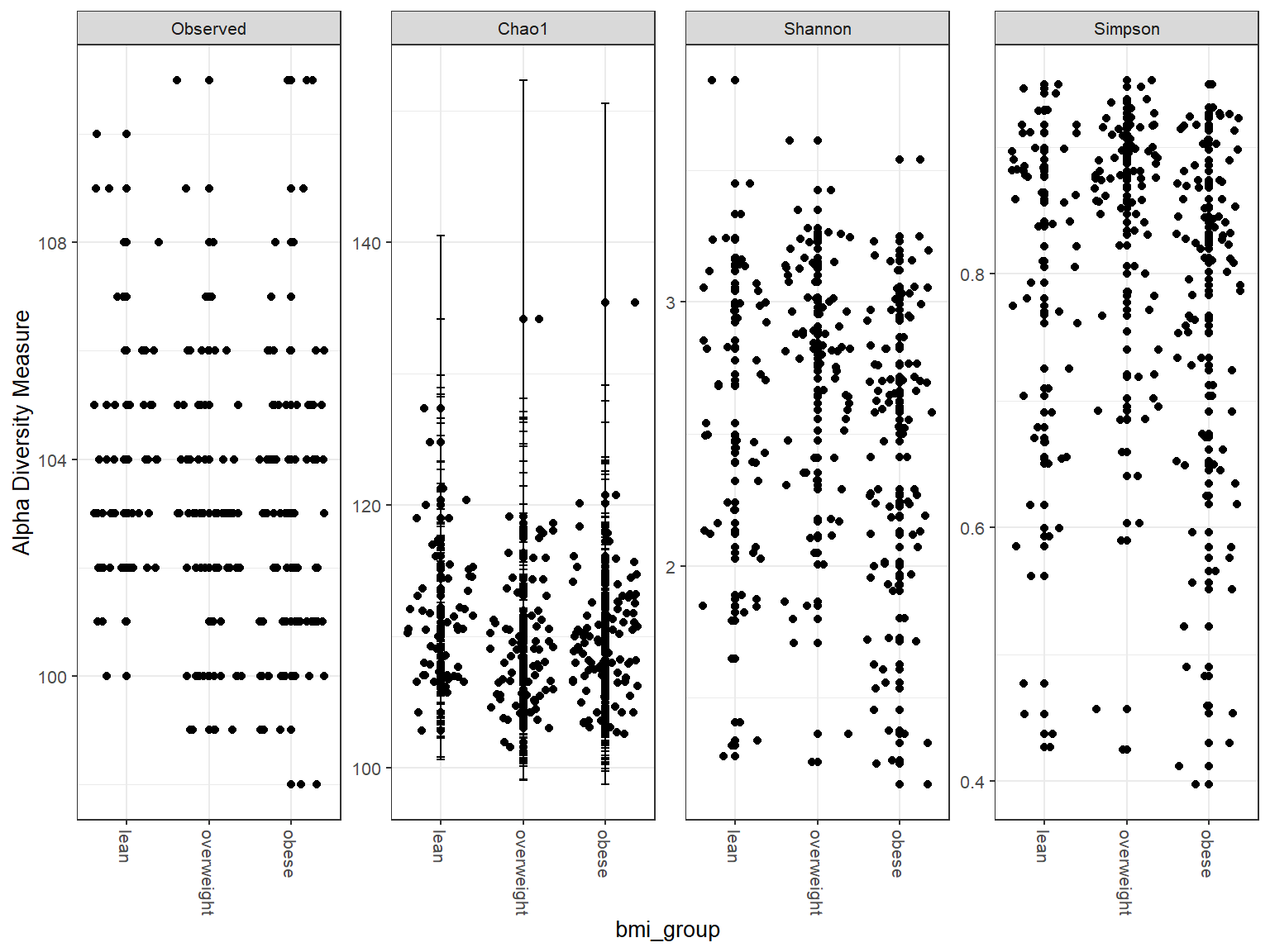
Violin plots

theme_set(theme_bw(10))
plot_richness(phy, x = "bmi_group", measures = alpha_metrics) + geom_violin(aes(fill = factor(bmi_group)),
    trim = FALSE, draw_quantiles = c(0.25, 0.5, 0.75)) + geom_jitter(height = 0,
    width = 0.1)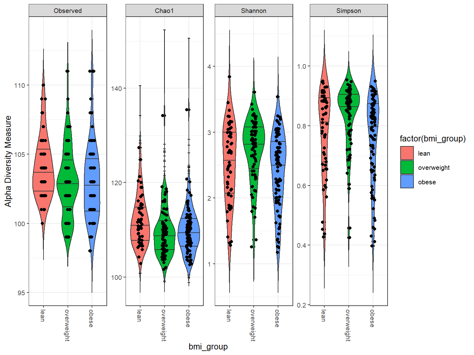

Part 2: non-parametric test

Kruskal-Wallis test

perform Kruskal-Wallis test between bmi_groups, since it has three factors. The purpose behind the test would be more clear.

alphas <- estimate_richness(phy, measures = alpha_metrics)
kw <- t(sapply(alphas, function(x) unlist(kruskal.test(x ~ sample_data(phy)$bmi_group)[c("p.value",
    "statistic")])))
kw

             p.value statistic.Kruskal-Wallis chi-squared
Observed 0.022081536                             7.626027
Chao1    0.015152446                             8.379187
se.chao1 0.025379869                             7.347598
Shannon  0.001053162                            13.711917
Simpson  0.001623541                            12.846291

As Kruskal-Wallis test is significant

Post hoc

Post hoc by implementing Conover’s test

Using shannon index

df <- cbind(get_variable(phy), alphas$Shannon)

library("conover.test")

con <- conover.test::conover.test(df$`alphas$Shannon`, df$bmi_group, kw = T, method = "bonferroni")

  Kruskal-Wallis rank sum test

data: x and group
Kruskal-Wallis chi-squared = 13.7119, df = 2, p-value = 0

                           Comparison of x by group                            
                                 (Bonferroni)                                  
Col Mean-|
Row Mean |       lean      obese
---------+----------------------
   obese |   1.177492
         |     0.3604
         |
overweig |  -2.205510  -3.779721
         |     0.0427    0.0003*

alpha = 0.05
Reject Ho if p <= alpha/2

Using Simpson index

df1 <- cbind(get_variable(phy), alphas$Simpson)

con1 <- conover.test::conover.test(df1$`alphas$Simpson`, df1$bmi_group, kw = T, method = "bonferroni")

  Kruskal-Wallis rank sum test

data: x and group
Kruskal-Wallis chi-squared = 12.8463, df = 2, p-value = 0

                           Comparison of x by group                            
                                 (Bonferroni)                                  
Col Mean-|
Row Mean |       lean      obese
---------+----------------------
   obese |   1.099905
         |     0.4089
         |
overweig |  -2.162227  -3.646024
         |     0.0475    0.0005*

alpha = 0.05
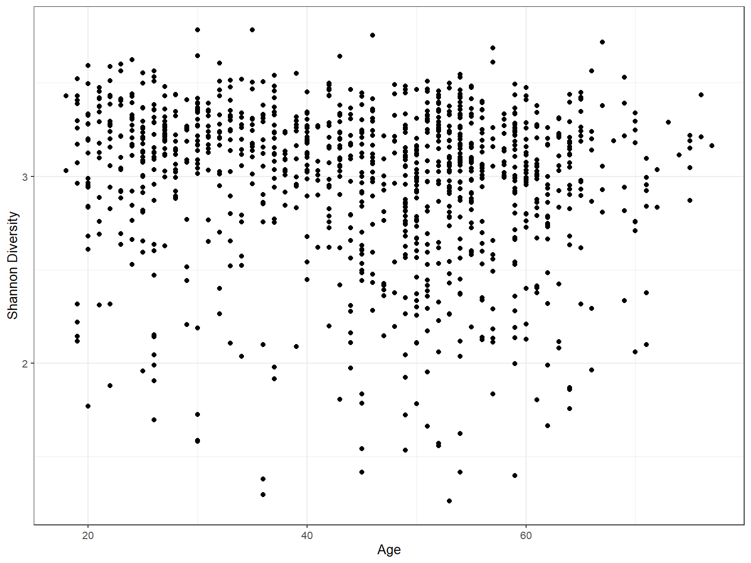
Reject Ho if p <= alpha/2

Part 3: Linear regression

Using another phyloseq dataset from micorobiome package, this phyloseq has continuous variable among its metadata variables. We shall see the linear regression for the diversity_shannon as a dependent variable on the ‘age’ as the independent variable.

atlas1006

This data set contains genus-level microbiota profiling with HITChip for 1006 western adults with no reported health complications, reported in Lahti et al. (2014) https://doi.org/10.1038/ncomms5344.

phyloseq-class experiment-level object
otu_table()   OTU Table:         [ 130 taxa and 1151 samples ]
sample_data() Sample Data:       [ 1151 samples by 10 sample variables ]
tax_table()   Taxonomy Table:    [ 130 taxa by 3 taxonomic ranks ]

Linear regression model.

Analysis of Variance Table

Response: diversity$Shannon
            Df  Sum Sq Mean Sq F value    Pr(>F)    
age          1   3.167  3.1666  18.406 1.943e-05 ***
Residuals 1093 188.045  0.1720                      
---
Signif. codes:  0 '***' 0.001 '**' 0.01 '*' 0.05 '.' 0.1 ' ' 1

It is significant p_value

Regression plot

Acknowledgement An Introduction to Statistical Learning

regplot = function(x, y, ...) {
    fit = lm(y ~ x)
    plot(x, y, ...)
    abline(fit, col = "red")
}

attach(data)
regplot(x = age, y = diversity$Shannon, xlab = "Age", ylab = "Shannon Diversity",
    pch = 20)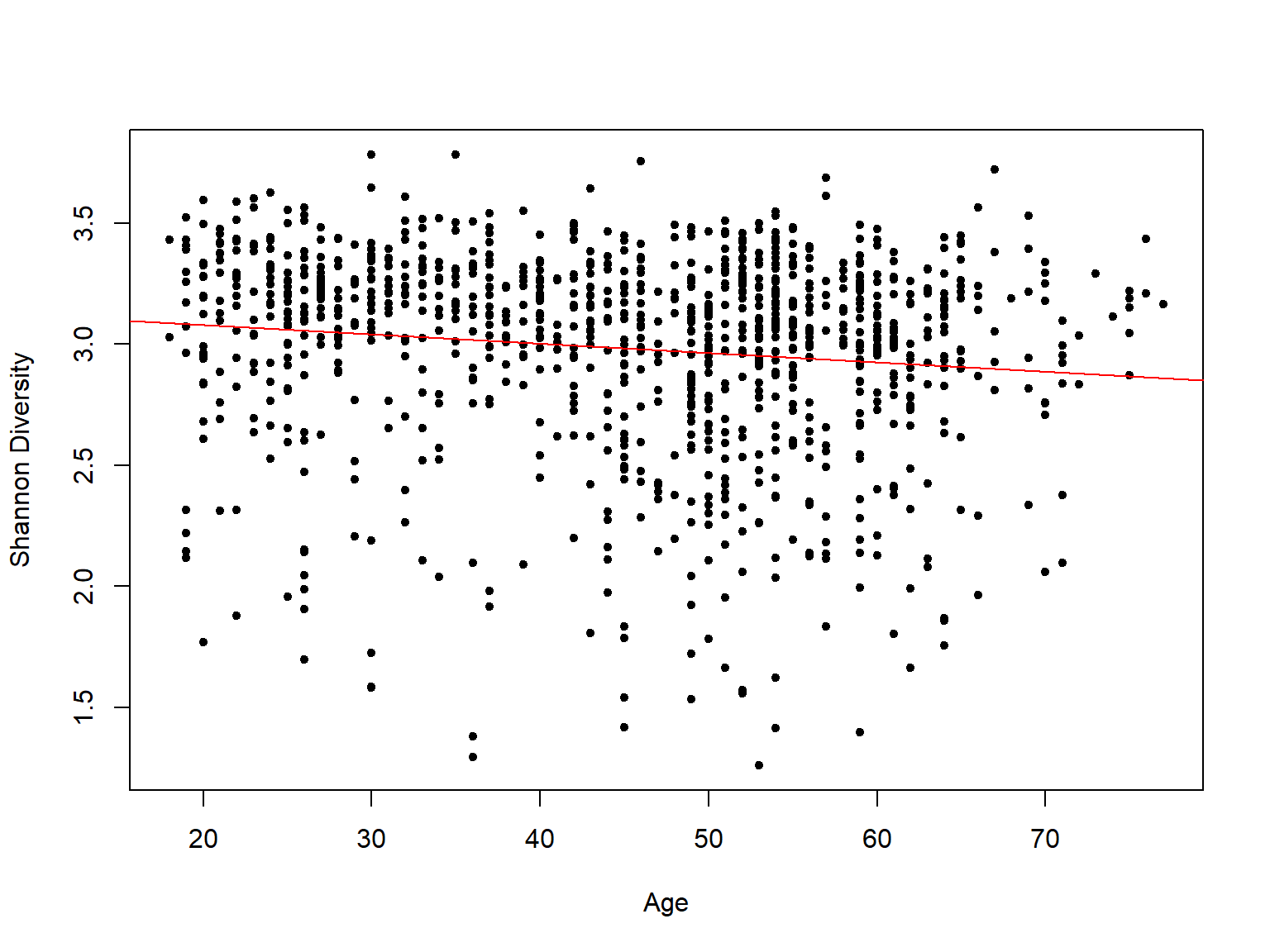

Important In microbiome analysis we do not check the normality conditions by Shapiro test for example, it is enough to check the histograms and see the pattern of the continuous variable.